

Introduction
Most R code I inherit has the same shape: a for loop, an accumulator initialised to NULL, and an if inside the loop that quietly does something different on the third iteration. It works. It’s also nearly impossible to test, because no piece of it is small enough to test on its own.
purrr is the tidyverse’s answer to that. It gives you a family of functions that apply one function across a list and hand back something whose type you can predict, which sounds modest until you’ve spent an afternoon working out why sapply() returned a matrix instead of a vector.
This post covers the map() family, the error wrappers I reach for most, and a few examples with real shapes: reading a directory of CSVs, fitting a model per group, generating a plot per subset. If you already write lapply() everywhere, some of this will look like a rename. The parts that aren’t a rename are the ones worth your time.
What functional programming actually buys you
The one-line version: write functions that take inputs and return outputs, and don’t let them touch anything else.
That constraint sounds academic. It isn’t. A function with no side effects returns the same answer every time you run it, so you can test it on its own, and the order you call things in stops mattering. Most of the debugging time I’ve lost in R has gone on the opposite: a variable modified three scopes away, or a loop whose result depended on what happened to be left in the environment from the previous run.
Two things follow from it.
Small functions are testable functions. Break a hundred-line pipeline into six named steps and you can check each against a handful of inputs. Leave it as one block and your only test is whether the whole thing crashed.
Avoiding explicit loops also nudges you toward vectorised operations, which in R are the fast path. That’s a side benefit rather than the point, but it’s a real one.
What purrr is
purrr is part of the tidyverse, and its job is applying functions over lists without the type surprises base R hands you.
The naming is what I’d point at first. map() returns a list. map_dbl() returns a double vector. map_chr() returns a character vector. That suffix is a contract: if your function returns something else, you get an error on that line rather than a confusing one four steps later. sapply() simplifies to whatever it feels like, and I’ve been caught by that on data where the first group happened to have exactly one row.
Beyond the naming, it handles nested structures without you flattening them by hand, it has real error handling (which gets its own section below), and it composes with dplyr and tidyr because it was built alongside them.
It’s on CRAN.
install.packages("purrr")
library(purrr)
The rest of this post is the functions themselves, with examples you can paste.
The functions worth knowing
Four things cover most of what I use purrr for. The map() family, pmap() for when several arguments vary together, the three error wrappers, and a couple of list utilities.
A. The map() family
This is the part you’ll use every day. map() takes a list and a function, applies the function to each element, and returns a list the same length. The variants differ only in what they promise to return, and that promise is the whole value: map_dbl() will error rather than quietly hand you a list.
map(): Returns a list.map_lgl(): Returns a logical vector.map_int(): Returns an integer vector.map_dbl(): Returns a double vector.map_chr(): Returns a character vector.map_df(): Returns a data frame.
Example:
# Define a list of numbers
number_list <- list(1, 2, 3, 4)

# Square each number using map()
squared_numbers <- map(number_list, ~ .x^2)
print(squared_numbers)
B. pmap()
pmap() is for when more than one thing varies. Give it a list of argument lists and it walks them in parallel, which beats writing a loop with three indices you have to keep aligned by hand.
Example:
# Define two lists
list1 <- list(1, 2, 3)
list2 <- list(4, 5, 6)

# Add corresponding elements of the two lists using pmap()
sum_list <- pmap(list(list1, list2), ~ ..1 + ..2)
print(sum_list)
C. safely(), quietly(), and possibly()
Is this worth a whole section? If you have ever lost a two-hour batch job to one malformed file at element 400, yes. This is the part I’d read first if you’re processing files or hitting an API. In a loop, one bad element kills the whole run and you lose everything before it. These three wrappers turn a failure into a value you can inspect afterwards, so the run finishes and you find out what broke at the end rather than at element 400 of 2,000.
safely(): Returns a list containing the result and any error encountered.quietly(): Returns a list containing the result, any warnings, and any messages.possibly(): Returns a default value if an error is encountered.
Example:
# Define a list with numbers and a character
mixed_list <- list(1, 2, "a", 3)

# Define a safely wrapped square function
safe_square <- safely(~ .x^2)

# Apply the safe_square function to the mixed_list
results <- map(mixed_list, safe_square)
print(results)
D. compact() and compose()
compact() is used to remove NULL elements from a list, while compose() allows you to combine multiple functions into a single function.
Example:
# Define a list with NULL elements
null_list <- list(1, NULL, 2, NULL, 3)

# Remove NULL elements using compact()
clean_list <- compact(null_list)
print(clean_list)

# Compose two functions: square and increment
square <- function(x) x^2
increment <- function(x) x + 1
square_and_increment <- compose(increment, square)

# Apply the composed function to a number
result <- square_and_increment(3)
print(result)
That’s the core. What follows is the same functions on data with realistic shapes.
Practical examples with purrr
Four examples. Summary statistics across columns, a model per subgroup, a directory of CSVs read in one pass, and a plot per group.
A. Example 1: Calculating summary statistics for multiple variables
You have a data frame and you want the same set of statistics for every numeric column. The loop version needs a pre-allocated result and a counter. This version doesn’t.
# Load required packages
library(dplyr)
library(purrr)

# Create a sample data frame
data <- data.frame(
  var1 = rnorm(100, mean = 10, sd = 2),
  var2 = rnorm(100, mean = 20, sd = 5),
  var3 = rnorm(100, mean = 30, sd = 3),
  stringsAsFactors = FALSE
)

# Define a list of summary functions
summary_functions <- list(mean = mean, median = median, sd = sd)

# Calculate summary statistics for each variable using nested map functions
summary_stats <- map_dfr(summary_functions, ~ map_dfc(data, .x), .id = "Statistic")
print(summary_stats)
B. Example 2: Fitting multiple linear models for different subsets of data
Fitting one model per group is where purrr starts paying for itself. Split, map, and you have a list of models you can then map over again to pull out coefficients or R-squared, without ever writing an index.
# Load required packages
library(dplyr)
library(purrr)
library(broom)

# Split the mtcars dataset by the number of cylinders
mtcars_split <- mtcars %>% group_split(cyl)

# Define a function to fit a linear model and extract coefficients
fit_lm <- function(data) {
  model <- lm(mpg ~ wt, data = data)
  coef <- data.frame(tidy(model)) %>%
    select(term, estimate) %>%
    mutate(cyl = unique(data$cyl))
  return(coef)
}

# Apply the fit_lm function to each subset using map_dfr()
model_coefs <- map_dfr(mtcars_split, fit_lm)
print(model_coefs)
C. Reading Multiple CSV files with purrr
This is the case I use most often, and it’s also where safely() earns its keep: one malformed file in a directory of two hundred should not cost you the other 199.
# Define the directory containing the CSV files
csv_directory <- "path/to/your/csv/files"

# List all CSV files in the directory
csv_files <- list.files(csv_directory, pattern = "*.csv", full.names = TRUE)

# Define a function to read a CSV file and add a column with the filename
read_csv_with_filename <- function(file) {
  data <- read_csv(file)
  data <- data %>% mutate(filename = basename(file))
  return(data)
}

# Read all CSV files using map_dfr() and bind the results into a single data frame
combined_data <- map_dfr(csv_files, read_csv_with_filename)
We list the CSVs, define a reader, map it over the paths, then bind the results into one frame. Swap map() for map(safely(read_one)) and a bad file becomes a row you can inspect rather than an error that ends the run.
D. purrr and ggplot2
Same idea, different output. Instead of a list of models, you get a list of ggplot objects, one per group, which you can then arrange on a grid.
# Load required packages
library(purrr)
library(ggplot2)
library(dplyr)
library(cowplot)

# Create a list of data frames, one for each unique number of cylinders in the mtcars dataset
data_list <- mtcars %>%
  split(.$cyl)

# Define a function to create a ggplot for a given data frame
create_ggplot <- function(data) {
  ggplot(data, aes(x = mpg, y = hp)) +
    geom_point(aes(color = factor(gear)), size = 3) +
    labs(title = paste("Number of Cylinders:", unique(data$cyl)),
         x = "Miles per Gallon",
         y = "Horsepower") +
    theme_minimal() +
    theme(legend.title = element_blank()) +
    scale_color_discrete(name = "Gears")
}

# Create a list of ggplots using map()
ggplot_list <- data_list %>%
  map(create_ggplot)

# Combine the ggplots into a single plot using cowplot's plot_grid()
combined_plot <- plot_grid(plotlist = ggplot_list, ncol = 1, align = "v", rel_heights = c(1, 1, 1))

# Display the combined plot
print(combined_plot)
And this is what that one map call produces — a plot per cylinder group, drawn by the same function:
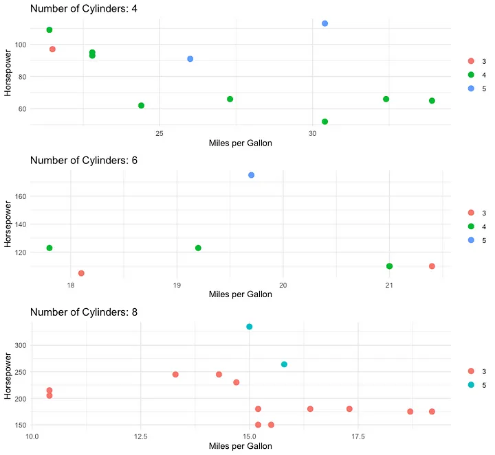
In this example, we first create a list of data frames, one for each unique number of cylinders in the mtcars dataset. Then, we define a custom function create_ggplot() to create a ggplot for a given data frame. The function creates a scatterplot of miles per gallon (mpg) versus horsepower (hp), with a title that reflects the number of cylinders.
Finally, we use purrr‘s map() function to apply the custom function to each data frame in the list, resulting in a list of ggplots. We use a for loop to display each ggplot.
The plot we get can be seen below:
In this example, we’ve made some changes to the create_ggplot() function to improve the aesthetics of the plots:
- We use
geom_point(aes(color = factor(gear)), size = 3)to color the points by the number of gears and increase their size. - We apply
theme_minimal()to use a minimalistic theme for the plots. - We remove the legend title using
theme(legend.title = element_blank()). - We rename the color scale to “Gears” using
scale_color_discrete(name = "Gears").
Finally, we use the plot_grid() function from the cowplot package to combine the ggplots in the ggplot_list into a single plot with one column and display the combined plot.
The pattern in all four is the same: name the operation you want to do once, then map it. What changes is what comes back.
Tips and Best Practices for Using purrr
A few things I’d tell someone picking this up.
1. Use anonymous functions when appropriate
When using map() functions, you can create anonymous functions using the ~ notation, which allows for concise and readable code. However, if the function becomes too complex or is used multiple times, consider defining it as a separate named function for better code organization and readability.
2. Compose functions instead of nesting them
compose() builds a new function out of existing ones, right to left. Two small named functions and a compose() beats one function doing both jobs, mostly because you can test each half.
3. Wrap anything that touches the outside world
Files, APIs, database calls: use safely(), quietly() or possibly(). A single bad element should cost you that element, not the run.
4. Know when to use purrr vs. base R or dplyr
While purrr provides a powerful and flexible way to manipulate data, there are cases where base R or dplyr functions may be more appropriate or efficient. For example, if you need to perform simple operations on a data frame, consider using dplyr functions like mutate() or summarize(). Evaluate the needs of your specific task and choose the best tool for the job.
5. Read the reference, not just the cheatsheet
There’s more in the package than the map() family, and the reference is short. imap(), walk() and reduce() are the three I wish I’d found sooner.
None of this is a rule. But if you write R for a living, the error wrappers alone will save you an afternoon within the month.
Wrapping up
purrr is a rename of lapply() right up until it isn’t. The map_*() suffixes stop type surprises at the line that caused them, pmap() removes the multi-index loop, and the error wrappers turn a crashed batch job into a result set with some failures in it.
If you take one thing: wrap anything that touches a file or a network in safely() before you run it over two thousand elements. I have learned that one the expensive way.
Happy coding.
Further reading
- The purrr reference — short, and the examples run.
- R for Data Science, Wickham and Grolemund. The iteration chapter is the gentlest introduction to this material anywhere.
- Advanced R, Wickham. Read the Functionals chapter when you want to know why
map()is built the way it is. - The Posit Community forum, if you are stuck on something specific.
Harnessing these resources and proactively mingling with the wider R circle will undoubtedly refine your prowess with both the
purrrpackage and R’s functional programming realm. Continue your journey of discovery, trial, and collaborative learning to blossom as an adept data scientist and R aficionado.
Artificial Intelligence Data Science functional programming Programming R Rstats