

Two R packages solve the same problem in opposite ways, and which one you should reach for depends on something most comparisons skip: how big the data is, and who else has to read the code.
The tidyverse optimises for the reader. data.table optimises for the machine. Both are excellent. I use both, usually in the same project, and the choice is rarely close once you know what you’re optimising for.
The tidyverse is a family of packages, dplyr, tidyr, ggplot2 and others, built around a shared grammar. Verbs read left to right, joined by a pipe, and someone who has never seen the code can usually tell what a chain does on first reading. That’s not a small thing when the person maintaining your analysis in a year is not you.
data.table trades that legibility for speed and memory. Its syntax is dense, it modifies in place rather than copying, and on a few million rows the difference stops being academic.
Same operations in both, below.
Examples: Tidyverse Examples
Here are some examples of how to use the tidyverse:
To select specific columns from a dataset:
# Load the tidyverse package
library(tidyverse)

# Load the mpg dataset from the ggplot2 package
data(mpg)

# Select the "manufacturer" and "model" columns
mpg %>% select(manufacturer, model)
And to group and summarize a dataset:
# Load the tidyverse package
library(tidyverse)

# Load the mpg dataset from the ggplot2 package
data(mpg)

# Group the dataset by "class" and compute the mean of the "hwy" column
mpg %>% group_by(class) %>% summarize(mean_hwy = mean(hwy))
To join two datasets:
# Load the tidyverse package
library(tidyverse)

# Load the mpg and cylinders datasets from the ggplot2 package
data(mpg)
data(cylinders)

# Join the mpg and cylinders datasets on the "manufacturer" column
mpg %>% left_join(cylinders, by = "manufacturer")
To perform a linear regression using the lm function from the stats package:
# Load the tidyverse and stats packages
library(tidyverse)
library(stats)

# Load the mtcars dataset
data(mtcars)

# Perform a linear regression to predict mpg (miles per gallon) using wt (weight) as the predictor variable
fit <- mtcars %>%
  lm(mpg ~ wt, data = .)

# Summarize the model results
summary(fit)
Create a scatterplot matrix using the scatterplotMatrix function from the car package:
# Load the tidyverse and car packages
library(tidyverse)
library(car)

# Load the iris dataset
data(iris)

# Create a scatterplot matrix of the iris dataset
scatterplotMatrix(iris, smooth = FALSE)
Create a faceted bar plot using ggplot2:
# Load the tidyverse package
library(tidyverse)

# Load the mpg dataset from the ggplot2 package
data(mpg)

# Create a faceted bar plot showing the distribution of hwy (highway miles per gallon) by class and drv (drive type)
ggplot(mpg, aes(x = hwy)) +
  geom_histogram(binwidth = 2) +
  facet_wrap(~ class + drv, nrow = 2)
Examples: data.table Examples
The data.table package, on the other hand, is a high-performance package for working with large datasets. It provides functions for manipulating and querying data efficiently. The data.table package is particularly useful when working with datasets that are too large to fit in memory or when you need to perform complex operations on large datasets.
One of the main advantages of the data.table package
One of the main advantages of the data.table package is its speed. The functions in the data.table package are generally faster than their counterparts in the tidyverse, especially when working with large datasets.
So I measured it rather than repeating it. Group by a letter, average a column, three sizes:
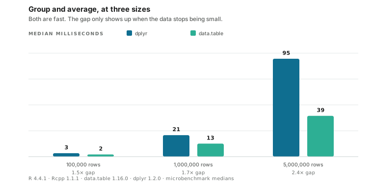
Both are fast, and that is the part the benchmark wars tend to skip. On a hundred thousand rows the difference is about a millisecond, so pick whichever you write more fluently. The gap only earns an opinion once the data stops being small, and then it widens rather than holding steady.
Here are some more examples of how to use the data.table package:
To select specific columns from a dataset:
# Load the data.table package
library(data.table)

# Load the mpg dataset from the ggplot2 package
data(mpg)

# Convert the dataset to a data.table
mpg <- as.data.table(mpg)

# Select the "manufacturer" and "model" columns
mpg[, .(manufacturer, model)]
and to group and summarize a dataset:
# Load the data.table package
library(data.table)

# Load the mpg dataset from the ggplot2 package
data(mpg)

# Convert the dataset to a data.table
mpg <- as.data.table(mpg)

# Group the dataset by "class" and compute the mean of the "hwy" column
mpg[, .(mean_hwy = mean(hwy)), by = class]
To join two datasets:
# Load the data.table package
library(data.table)

# Load the mpg and cylinders datasets from the ggplot2 package
data(mpg)
data(cylinders)

# Convert the datasets to data.tables
mpg <- as.data.table(mpg)
cylinders <- as.data.table(cylinders)

# Join the mpg and cylinders datasets on the "manufacturer" column
mpg[cylinders, on = "manufacturer"]
Perform a linear regression using the lm function from the stats package and the data.table package:
# Load the data.table and stats packages
library(data.table)
library(stats)

# Load the mtcars dataset
data(mtcars)

# Convert the dataset to a data.table
mtcars <- setDT(mtcars)

# Perform a linear regression to predict mpg (miles per gallon) using wt (weight) as the predictor variable
fit <- mtcars[, lm(mpg ~ wt)]

# Summarize the model results
summary(fit)
Create a scatterplot matrix using the scatterplotMatrix function from the car package and the data.table package:
# Load the data.table and car packages
library(data.table)
library(car)

# Load the iris dataset
data(iris)

# Convert the dataset to a data.table
iris <- as.data.table(iris)

# Create a scatterplot matrix of the iris dataset
scatterplotMatrix(iris, smooth = FALSE)
Create a faceted bar plot using ggplot2 and the data.table package:
# Load the data.table and ggplot2 packages
library(data.table)
library(ggplot2)

# Load the mpg dataset from the ggplot2 package
data(mpg)

# Convert the dataset to a data.table
mpg <- as.data.table(mpg)

# Create a faceted bar plot showing the distribution of hwy (highway miles per gallon) by class and drv (drive type)
ggplot(mpg, aes(x = hwy)) +
  geom_histogram(binwidth = 2) +
  facet_wrap(~ class + drv, nrow = 2)
In terms of implementation, both the tidyverse and data.table packages are written in R, but some of the functions in the data.table package are implemented in C for improved performance.
So which one?
Ask how big the data is, then ask who reads the code.
Under a million rows, with people who will maintain it after you, use the tidyverse. The chains read like sentences, the errors are legible, and the performance difference will not be what slows the project down. On a few million rows or more, data.table stops being an optimisation and becomes the difference between an analysis that runs and one that doesn’t. It modifies in place instead of copying, and once memory is the constraint that matters more than syntax.
Does it have to be one or the other? No. dtplyr gives you dplyr verbs on a data.table backend, which is a reasonable middle if your team knows one syntax and your data has outgrown it.
At Analytica
We work in gigabytes to terabytes, so data.table is the default here and the tidyverse gets used for the plotting and the final report. That’s a consequence of our data sizes, not a verdict on the packages. Your constraint is probably different from ours, and it should decide this rather than anyone’s preference.