

Four rules. No player. That’s the entire specification of Conway’s Game of Life, and it is enough to build a pattern that computes.
John Conway published it in 1970. It’s a cellular automaton: a grid where each cell is alive or dead, and every cell’s next state depends only on how many of its eight neighbours are currently alive. You set a starting arrangement and then you don’t touch it again. Everything after that is the rules running.
What makes it worth an afternoon is how little it takes to get complicated. Gliders that travel across the grid. Oscillators that return to their starting shape every few generations. Arrangements that grow without bound. People have built a working Turing machine out of it, which means the four rules below are, in a strict sense, capable of computing anything computable.
Below: the rules, then implementations in R and in Python, both short enough to read in one sitting.
Game Rules
The game rules are as follows:
- Any live cell with fewer than two live neighbors dies, as if by underpopulation.
- Any live cell with two or three live neighbors lives on to the next generation.
- Any live cell with more than three live neighbors dies, as if by overpopulation.
- Any dead cell with exactly three live neighbors becomes a live cell, as if by reproduction.
These rules are applied to each cell in the grid simultaneously, with the state of the cells in the next generation being determined based on the state of the cells in the current generation. The game continues in this way, with the state of the cells being updated in each generation.
The Game of Life can be implemented in many different ways, with the rules being applied to a two-dimensional grid, or to a one-dimensional “tape,” or even to a three-dimensional space. There are also many variations of the rules that have been explored, with different sets of rules leading to different patterns and behaviors in the game.
The Game of Life is capable of producing a wide range of patterns, depending on the initial configuration of the cells and the specific rules that are being used. Some patterns remain stable over time, while others may evolve and change over the course of the game.
Game Patterns
The classic starting shapes and their fates, from the original post:
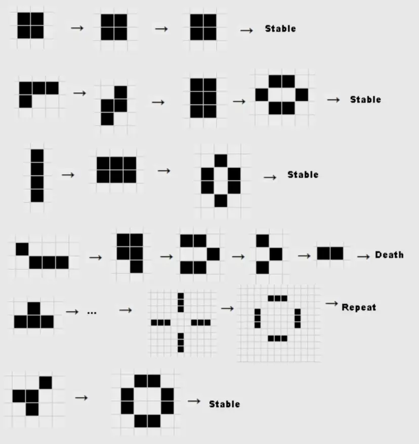
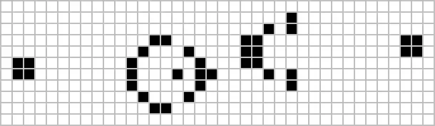
Few examples of patterns that can appear in the Game of Life
Here are a few examples of patterns that can appear in the Game of Life:
- Still lifes: These are patterns that remain stable over time and do not change from one generation to the next. Examples of still lifes include blocks, beehives, and loafs.
- Oscillators: These are patterns that repeat themselves over time, cycling through a fixed set of states. Examples of oscillators include blinkers, toads, and pulsars.
- Spaceships: These are patterns that move across the grid, leaving behind a “trail” of cells as they go. Spaceships can move in any of the four cardinal directions, and their movement may be periodic or aperiodic.
- Gliders: These are a type of spaceship that move diagonally across the grid, leaving behind a distinctive “trail” of cells. Gliders are one of the simplest and most well-known spaceships in the Game of Life.
- Guns: These are patterns that produce an endless stream of spaceships or other patterns. The first gun was discovered in 1970 by Bill Gosper, and many more have been found since.
- Patterns with complex behavior: Some patterns in the Game of Life exhibit behavior that is difficult to predict or understand. These patterns may exhibit seemingly random behavior, or they may exhibit complex, self-organizing behavior.
These are just a few examples of the patterns that can appear in the Game of Life. The game is capable of producing a wide range of patterns and behaviors, and new patterns are still being discovered today.
Real-Life Examples
So does any of this matter outside a screensaver? More than I expected when I first met it. The Game of Life turns up wherever people are trying to understand how local rules produce global behaviour.
- Biology: The Game of Life has been used to model the behavior of cellular automata, including the growth and division of cells. It has also been used to study patterns in the distribution of species in ecosystems and the spread of epidemics.
- Physics: The Game of Life has been used to model the behavior of physical systems, such as the formation of patterns in crystals and the behavior of fluids.
- Computer science: The Game of Life has been used as a test bed for exploring algorithms and data structures, and it has inspired the development of a number of computational models and techniques.
- Art and design: The Game of Life has inspired a number of artistic and design projects, including digital art, installations, and interactive exhibits.
- Education: The Game of Life has been used as a tool for teaching concepts in mathematics, computer science, and other fields, and it has been incorporated into educational software and curricula.
The thread running through all of those is the same one: nobody designed the glider. It falls out of the rules. That is the property people keep coming back for, and it is why I think every analyst should implement this once by hand.
Game Simulation in R
The script below simulates the Game of Life and produces a plot of the evolution of the cells over time. The plotly package is used to create an interactive heatmap, with “dead” cells being shown in darker shades and “alive” cells being shown in lighter shades. The x-axis of the plot represents the generation, and the y-axis represents the cell.
# Install the plotly and furrr packages if they are not already installed
# install.packages("plotly")
# install.packages("furrr")

library(plotly)
library(furrr)

# Set up the grid for the game
grid <- matrix(sample(c(0, 1), 100*100, replace = TRUE), nrow = 100)

# Initialize a list to store the state of the cells at each generation
grid_history <- rep(list(grid), generations)

# Simulate the game using the furrr package to parallelize the simulation
plan(multisession)
grid_history <- future_map(1:generations, function(i) {
  # Get the current state of the cells
  current_state <- grid_history[[i]]

  # Initialize the next state of the cells
  next_state <- matrix(0, nrow = nrow(current_state), ncol = ncol(current_state))

  # Iterate over each cell in the grid
  for (x in 1:nrow(current_state)) {
    for (y in 1:ncol(current_state)) {
      # Get the number of live neighbors for the current cell
      neighbors <- sum(current_state[max(x-1, 1):min(x+1, nrow(current_state)),
                                     max(y-1, 1):min(y+1, ncol(current_state))]) - current_state[x, y]

      # Apply the rules of the Game of Life to determine the next state of the cell
      if (current_state[x, y] == 1) {
        if (neighbors < 2 || neighbors > 3) {
          next_state[x, y] <- 0
        } else {
          next_state[x, y] <- 1
        }
      } else {
        if (neighbors == 3) {
          next_state[x, y] <- 1
        } else {
          next_state[x, y] <- 0
        }
      }
    }
  }

  # Update the state of the cells
  grid <- next_state

  # Store the state of the cells at the current generation
  grid
})

# Plot the evolution of the cells over time using the plotly package
plot_ly(z = grid_history, colorscale = "Blackbody", type = "heatmapgl") %>%
  layout(xaxis = list(title = "Generation"), yaxis = list(title = "Cell"))
Game Simulation in Python
The script below simulates the Game of Life and produces a plot of the evolution of the cells over time. The matplotlib package is used to create a heatmap, with “dead” cells being shown in darker shades and “alive” cells being shown in lighter shades. The x-axis of the plot represents the generation, and the y-axis represents the cell.
import numpy as np
import matplotlib.pyplot as plt

# Set up the grid for the game
grid = np.random.choice([0, 1], size=(100, 100))

# Initialize a list to store the state of the cells at each generation
grid_history = [grid]

# Simulate the game
for i in range(generations):
    # Get the current state of the cells
    current_state = grid_history[i]

    # Initialize the next state of the cells
    next_state = np.zeros((100, 100))

    # Iterate over each cell in the grid
    for x in range(100):
        for y in range(100):
            # Get the number of live neighbors for the current cell
            neighbors = (current_state[max(x-1, 0):min(x+2, 100), max(y-1, 0):min(y+2, 100)]).sum() - current_state[x, y]

            # Apply the rules of the Game of Life to determine the next state of the cell
            if current_state[x, y] == 1:
                if neighbors < 2 or neighbors > 3:
                    next_state[x, y] = 0
                else:
                    next_state[x, y] = 1
            else:
                if neighbors == 3:
                    next_state[x, y] = 1
                else:
                    next_state[x, y] = 0

    # Update the state of the cells
    grid = next_state

    # Store the state of the cells at the current generation
    grid_history.append(grid)

# Plot the evolution of the cells over time using the matplotlib package
plt.imshow(grid_history, cmap="Greys")
plt.xlabel("Generation")
plt.ylabel("Cell")
plt.show()
Why it’s worth your time
Four rules and no player, and you get gliders, oscillators, and arrangements that grow forever. That gap between how simple the specification is and how complicated the behaviour gets is the whole reason people still write these implementations forty-odd years on.
It’s also a useful thing to keep in mind when you build models for a living. Complicated output does not require a complicated model. Sometimes it requires four rules and enough iterations, which is worth remembering the next time somebody insists a phenomenon must have a complicated cause.
Run either script above and change the starting grid. That’s the fun part.